Data Cleaning, Wrangling, and Exploration

Load files

Code

library(tidyverse) 
library(stringr) 
library(geomtextpath) # for annotating geom_vlines
library(mosaic, include.only = 'favstats')
library(knitr, include.only='kable')
library(eyetrackingR) # add_aoi, need equal time windows
library(wesanderson)

list_of_files_with_ID <- list.files(path = "data_5/",
                            recursive = TRUE,
                            pattern = "\\.csv$",
                            full.names = TRUE)
# writeLines(list_of_files, "filenames.txt")

df <- list_of_files_with_ID %>% setNames(nm = .) %>%
  map_df(~read_csv(file = .x, col_types = cols()), .id = "participant") %>%
           mutate(participant = str_extract(participant, "V\\d{3}")
                  )
# above did not work with baseR pipe |>, had to use the tidy pipe

Examine validation scores

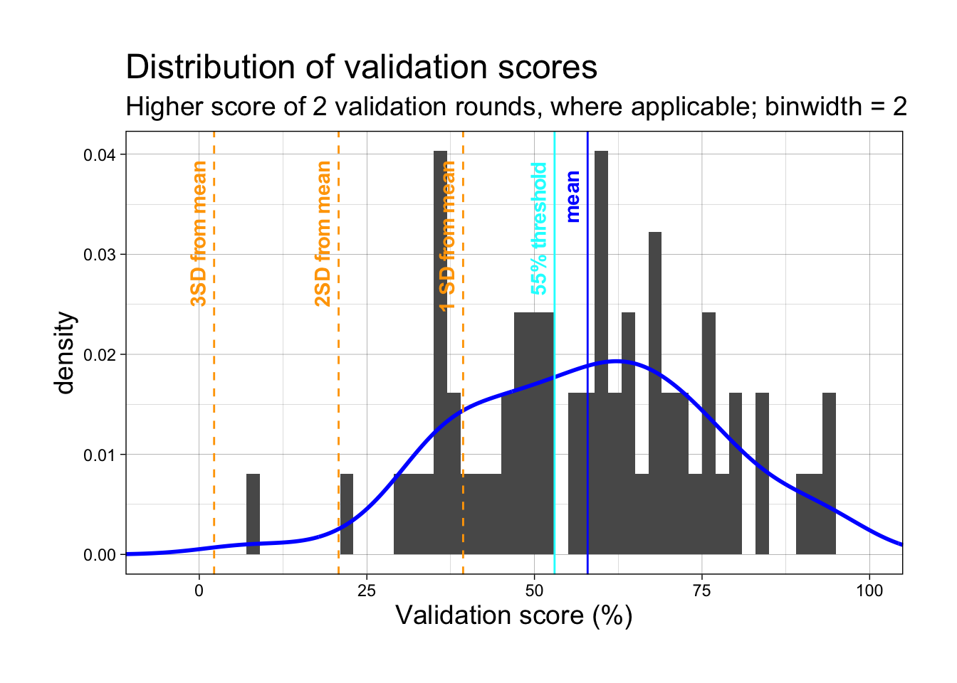
Validation scores are calculated percent_in_roi column.

The preregistered exclusion method is 55% validation accuracy within 2 rounds (gaze falls within 200px radius of 5 validation points).

Code

# column percent_in_roi has brackets [], function to remove
remove_brackets <- function(col) {
  gsub("\\[|\\]", "", col)
}

# percent_in_roi originally is a string, e.g., "[100, 100, 100, 100, 100]"
# remove brackets, str_split into list of 5 strings, e.g., c("100", "100", "100", "100", "100")
df_percent_in_roi <- df |> group_by(participant) |> 
  select(participant, percent_in_roi) |> drop_na() |> 
  mutate(percent_in_roi = remove_brackets(percent_in_roi)) |> 
  mutate(list_percent = str_split(percent_in_roi, ","))

# split the list of string into 5 columns, for each column, as.numeric()
df_calculate_mean <- df_percent_in_roi |> select(participant, list_percent) |> unnest_wider(list_percent, names_sep = ".") |>
mutate_at(c('list_percent.1', 'list_percent.2', 'list_percent.3', 'list_percent.4', 'list_percent.5'), as.numeric) |> 
  # calculate means for each row, i.e., each round of validation
  # create boolean column to indicate whether participants passed 55% threshold or not
  mutate(
  mean_col = rowMeans(cbind(list_percent.1, list_percent.2, 
                            list_percent.3, list_percent.4, 
                            list_percent.5), na.rm=F)) |> 
  mutate(boolean = case_when(mean_col >= 55.0 ~ TRUE, 
                             mean_col < 55 ~ FALSE))

rmarkdown::paged_table(head(df_calculate_mean, n=10))

Get higher validation score for participants, if 2 rounds of validation

Code

# generate participant list who reach 55% within 2 rounds of validation
# retain rows with higher validation percent in mean_col,  using top_n()
participant_list_eye_tracking <- df_calculate_mean |> 
  group_by(participant) |> top_n(1, mean_col)

rmarkdown::paged_table(head(participant_list_eye_tracking))

Quick calculation: what if we were to use “validation score above 80% on any of 5 points”

Code

q <- participant_list_eye_tracking |> 
  mutate(max_percent_of_single_point = max(c(list_percent.1, list_percent.2, list_percent.3, list_percent.4, list_percent.5))) |> 
  mutate(above_80 = case_when(
    max_percent_of_single_point >= 80 ~TRUE, 
    max_percent_of_single_point < 80 ~ FALSE
  ))

q |> group_by(above_80) |> count()

# A tibble: 2 × 2
# Groups:   above_80 [2]
  above_80     n
  <lgl>    <int>
1 FALSE        8
2 TRUE        54

FALSE 8
TRUE 54
Conclusion: If we use the approach of 80% score on any validation point, then we would only exclude 8 participants.

Subset for participants who passed the threshold

narrow_participant_list_eye_tracking is the list of participants whose data we will use for eye-tracking analysis.

Code

# subset data of participants who passed the validation score threshold
narrow_participant_list_eye_tracking <- participant_list_eye_tracking |> filter(boolean == TRUE)

rmarkdown::paged_table(head(narrow_participant_list_eye_tracking))

Descriptive statistics of all participants

Code

# descriptive stats on mean_col of ALL participants
descriptive_stats_mean_validation_scores <- favstats(~mean_col, data = participant_list_eye_tracking)

knitr::kable(descriptive_stats_mean_validation_scores, align = "c", 
             caption = "Descriptive statistics, validation scores of all participants")

Descriptive statistics, validation scores of all participants

	min	Q1	median	Q3	max	mean	sd	n	missing
	7.567568	45.59098	59.43423	70.03414	94.59459	57.93148	18.57287	62	0

Histogram and density curve of all participants

Code

ggplot(participant_list_eye_tracking, aes(x=mean_col)) + 
  #set histogram and density plot
  geom_histogram(aes(y = after_stat(density)), binwidth = 2) + 
  geom_density(color="blue", linewidth = 1) +
  #set theme
  theme_linedraw() +
    theme(
        plot.margin = margin(1,1,1,1, "cm"), 
        plot.title = element_text(size=18), 
        plot.subtitle = element_text(size=14), 
        axis.title = element_text(size = 14)
        ) +
  # add vlines to indicate mean, SD from mean, and where the 55% threshold is
  # using geomtextpath::geom_textvline which combines vline and annotation settings
  # mean
    geom_textvline(label = "mean", xintercept = mean(participant_list_eye_tracking$mean_col), 
                   color = "blue", vjust = -.5, hjust = .9, fontface = "bold") +
    geom_textvline(label = "3SD from mean", xintercept = (mean(participant_list_eye_tracking$mean_col) - sd(participant_list_eye_tracking$mean_col)*3), 
                   color = "orange", vjust = -.5, linetype="dashed", hjust = .9, fontface = "bold") +
    geom_textvline(label = "2SD from mean", xintercept=(mean(participant_list_eye_tracking$mean_col) - sd(participant_list_eye_tracking$mean_col)*2), 
                   color = "orange", vjust = -.5, linetype="dashed", hjust = .9, fontface = "bold") +
    geom_textvline(label = "1 SD from mean", xintercept=(mean(participant_list_eye_tracking$mean_col) - sd(participant_list_eye_tracking$mean_col)), 
                   color = "orange", vjust = -.5, linetype="dashed", hjust = .9, fontface = "bold") + 
  #55% threshold
  geom_textvline(label = "55% threshold", xintercept = 53, color = "cyan", vjust = -.5, hjust = .9, fontface = "bold") +
# set plot titles
  ggtitle("Distribution of validation scores", subtitle = "Higher score of 2 validation rounds, where applicable; binwidth = 2") + 
# set axis labels
  scale_x_continuous(name = "Validation score (%)", limits=c(-11, 105), expand = c(0, 0))

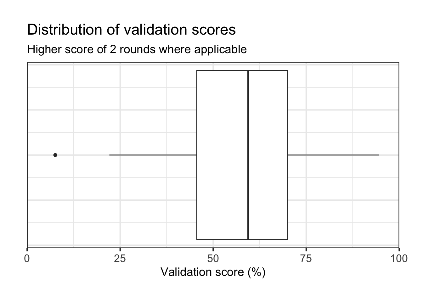
Box and whisker plot, validation scores of all participants

Code

ggplot(participant_list_eye_tracking, aes(x = mean_col))+
  geom_boxplot() +
  scale_x_continuous(name = "Validation score (%)", 
                     limits=c(0, 100), 
                     expand = c(0, 0)) + 
  theme_bw(base_size=16) +
  theme(axis.text.y = element_blank(), 
        axis.ticks.y = element_blank(),
        plot.margin = margin(1,1,1,1, "cm"), 
        plot.title = element_text(size=18), 
        plot.subtitle = element_text(size=14), 
        axis.title = element_text(size = 14)) +  
    ggtitle("Distribution of validation scores", subtitle = "Higher score of 2 rounds where applicable")

Descriptive statistics for each validation point

Code

#table for each validation point, mean, sd of validation scores

m1 <- favstats(narrow_participant_list_eye_tracking$list_percent.1) |> mutate(point ="[25, 25]", .before = min)
m2 <- favstats(narrow_participant_list_eye_tracking$list_percent.2) |> mutate(point ="[75, 25]", .before = min)
m3 <- favstats(narrow_participant_list_eye_tracking$list_percent.3) |> mutate(point ="[50, 50]", .before = min)
m4 <- favstats(narrow_participant_list_eye_tracking$list_percent.4) |> mutate(point ="[25,75]", .before = min)
m5 <- favstats(narrow_participant_list_eye_tracking$list_percent.5) |> mutate(point ="[75, 75]", .before = min)

#descriptive stats for each validation point
each_validation_point <- rbind(m1, m2, m3, m4, m5) 
rownames(each_validation_point) <- NULL #turn off automatically assigned row names

knitr::kable(each_validation_point, align="c", 
             caption = "**Participants who passed the 55% threshold, validation scores on each data point**")

Participants who passed the 55% threshold, validation scores on each data point

point	min	Q1	median	Q3	max	mean	sd	n	missing
[25, 25]	0.00000	85.78579	96.21859	100.00000	100	85.91404	23.22511	36	0
[75, 25]	0.00000	56.69643	80.81832	97.44521	100	69.97007	31.27701	36	0
[50, 50]	35.13514	82.00140	92.43717	100.00000	100	86.81598	16.32402	36	0
[25,75]	0.00000	15.54054	73.76931	90.29680	100	55.71681	39.47861	36	0
[75, 75]	0.00000	12.58600	65.68034	88.51351	100	55.20860	38.92314	36	0

Reaction time data

Cleanup

Code

remove_brackets <- function(col) {
  gsub("\\[|\\]", "", col)
}

# load data on the frame just before liquid appears, in milliseconds
frame_before_outcome <- read_csv("ReactionTime_FrameBeforeOutcome.csv")

df_reaction_time <- df |> select(participant, trial_index, rt, stimulus, response) |> drop_na()

reactionTime <- df_reaction_time |>
  filter(trial_index > 14)  |> # remove NA due to on-screen instructions appeared before trial_index 14 (response not captured)
  filter(trial_index != 16) |> 
  filter(stimulus != "img/plus_thin.png") |> # remove NA during fixation cross
  filter(!grepl('>', stimulus)) |> 
  mutate(stimulus = remove_brackets(stimulus)) |> # remove brackets
  mutate(stimulus = gsub("\\..*", "", stimulus)) |> #remove file extension .mp4
  mutate(stimulus = gsub(".*/","", stimulus)) |> #remove filepath videos/
  #rename the human stimuli as file names too terse
  mutate(stimulus = str_replace_all(stimulus, pattern = "HBC", replacement = "HumanBioCorrect")) |> 
  mutate(stimulus = str_replace_all(stimulus, pattern = "HBS", replacement = "HumanBioSpill")) |> 
  mutate(stimulus = str_replace_all(stimulus, pattern = "HNBC", replacement = "HumanNonbioCorrect")) |> 
  mutate(stimulus = str_replace_all(stimulus, pattern = "HNBS", replacement = "HumanNonbioSpill")) |>
  group_by(participant) |> 
  mutate(trial_index = dense_rank(desc(trial_index))) |> ungroup() |> 
# add column to indicate if the condition was "Correct" (f) or "Error" (j)
# the stimulus names (video file names) contains the string "Spill" or "Correct"
mutate(correct_answer = case_when(
  str_detect(stimulus, "Spill") ~ "j", str_detect(stimulus, "Correct") ~ "f")) |>
# reaction time data were saved by jsPsych as string, we convert to numeric
  mutate(rt = as.numeric(rt))  |> 
# join with csv frame_before_outcome loaded above 
  full_join(frame_before_outcome) |> 
# add column to calculate how much in advance participants gave key-press response
  mutate(rt.adjusted = (pour_moment - rt)) |> 
  # add column of booleans comparing whether participants' answers were correct
  mutate(accuracy = case_when(
  (response == correct_answer) ~ TRUE, 
  (response != correct_answer) ~ FALSE
), .before = pour_moment)

rmarkdown::paged_table(head(reactionTime, n = 15))

Calculate accuracy rate for each participant

Code

# group_by participant to work on exclusion 3
accuracy_for_each_participant <- reactionTime |> group_by(participant, accuracy) |> count() |> 
  mutate(percent_accuracy = n / 36 * 100) |> filter(accuracy == TRUE)

rmarkdown::paged_table(head(accuracy_for_each_participant))

Apply exclusions (Exclusion 3 -> 2 -> 1)

Exclusions as preregistered 1) exclude implausible reaction times (implausible = react within first 25% of video time) 2) exclude those who fail to give a key-press response for > 20% of videos (i.e., more than 7 trials), indicate distraction or misunderstood instructions. 3) exclude participants > 20% misjudgment, i.e., < 80% accuracy

Exclusion 3

Exclude participants who got < 80% accuracy overall, i.e., judged 8 videos wrong

Code

low_accuracy_participants <- accuracy_for_each_participant |> filter(percent_accuracy < 80)
# excluding 3 people (so far)
# participants V14, V39, V52 will be excluded

# copy the main df to play around
reactionTime_copy <- reactionTime

reactionTime_copy <- reactionTime_copy |> filter(!grepl('V014|V039|V052', participant))

Exclusion 2

Exclude participants who gave more than 7 NULL key-press responses

We can see that the highest number of NULL response (i.e., participants gave no key-press response during stimuli) was 3 trials. Nobody is excluded on Exclusion 2!

Code

na_in_response_time <- reactionTime_copy |> 
  mutate(na_response_time = !is.na(reactionTime_copy$rt.adjusted)) |> 
  group_by(participant, na_response_time) |> count() |> 
  # if we 
  filter(na_response_time == FALSE) |> arrange(desc(n))

rmarkdown::paged_table(head(na_in_response_time))

Exclusion 1

Exclude implausible reaction times (replace with NA) Here we are excluding data, not participants.

Code

process_implausible_reaction_times <- reactionTime_copy |> select(participant, trial_index, rt, pour_moment) |> 
  # responding during first 25% of movement is considered implausible
  mutate(implausible = pour_moment/4) |>  
  mutate(rt_implausible = case_when(rt <implausible ~ "replace_with_na", 
                                    rt >= implausible ~ "include"))

# if we examine the column rt_implausible, we see that only 1 participant had 1 implausible
examine_implausble <- process_implausible_reaction_times |> filter(rt_implausible == "replace_with_na")

# CAUTION: Dataframe modified in place. 
reactionTime_copy <- reactionTime_copy |> 
  mutate(rt = replace(rt, participant=="V015" & trial_index==2, NA), 
         rt.adjusted = replace(rt.adjusted, participant=="V015" & trial_index==2, NA))

Treatment of late responses and wrong responses

Wrong responses become NAs

Code

reactionTime_remove_wrongResponse <- reactionTime_copy |> 
  mutate(response_time_for_analysis = case_when(accuracy == FALSE ~ NA,
                            accuracy == TRUE ~ rt.adjusted))
#sum(!complete.cases(reactionTime_remove_wrongResponse$response_time_for_analysis))
# out of 60 participants
# 192 wrong responses removed out of 2161 trials
# 8.8% of responses were wrong

Code

reactionTime_preprocess <- reactionTime_remove_wrongResponse |>
  filter(stimulus != "Practice_dog_medium") |> 
  select(-c(trial_index, rt, response, correct_answer, accuracy, pour_moment, 
            rt.adjusted)) |> 
  group_by(participant, stimulus) |> 
# calculate mean for 3 rounds of participants' response times
  mutate(mean_of_3_rounds = mean(response_time_for_analysis, na.rm = TRUE)) |>
# filter(!is.nan(mean_of_3_rounds)) |> 
  select(-response_time_for_analysis) |> distinct() |>
# after combining into mean, only 1 data point was NA
# sum(!complete.cases(reactionTime_preprocess$mean_of_3_rounds)) # 1
# create columns for different conditions, for plotting
  mutate(agent = case_when(
    str_detect(stimulus, "Human") ~ "Human", 
    str_detect(stimulus, "Milo") ~ "Humanoid", 
    str_detect(stimulus, "Theo") ~ "Robotic Arm", 
  )) |> 
  mutate(motion_type = case_when(
    str_detect(stimulus, "Bio") ~ "Biological",
    str_detect(stimulus, "Nonbio") ~ "Nonbiological", 
  )) |>
  mutate(outcome_type = case_when(
    str_detect(stimulus, "Correct") ~ "Correct", 
    str_detect(stimulus, "Spill") ~ "Error"
  )) |> filter(stimulus != "Practice_medium_dog") |> 
    mutate(stimulus = factor(stimulus, 
                           levels=c("TheoBioCorrect", "TheoBioSpill", 
                                    "TheoNonbioCorrect", "TheoNonbioSpill", 
                                    "MiloBioCorrect", "MiloBioSpill", 
                                    "MiloNonbioCorrect", "MiloNonbioSpill", 
                                    "HumanBioCorrect", "HumanBioSpill", 
                                    "HumanNonbioCorrect", "HumanNonbioSpill")))



reactionTime_preprocess <- reactionTime_preprocess |> 
  mutate(mean_of_3_rounds = case_when(mean_of_3_rounds < -200 ~ NA, 
                                      TRUE ~ mean_of_3_rounds)) 

# participants to be excluded due to late responses: 7 people
#2, 4, 8, 16, 17, 32, 34

reactionTime_preprocess <- reactionTime_preprocess |> 
  filter(!participant %in% c("V002", "V004", "V008", 
                          "V016", "V017", "V032", "V034"))

sum(!complete.cases(reactionTime_preprocess$mean_of_3_rounds)) #92

[1] 92

Code

#52 participants remaining

Impute mean of each stimulus for the NAs

Code

reactionTime_impute <- reactionTime_preprocess |> group_by(stimulus) |> 
  summarise(stimulus_mean = mean(mean_of_3_rounds, na.rm = TRUE))

# HumanBioCorrect 141.0958333
# HumanBioSpill 332.0512821
# HumanNonbioCorrect 184.2254902
# HumanNonbioSpill 321.3233333
# 
# MiloBioCorrect 413.3137255
# MiloBioSpill 542.9198718
# MiloNonbioCorrect 16.7849462
# MiloNonbioSpill 0.7849462
# 
# TheoBioCorrect 373.8472222
# TheoBioSpill 520.4519231
# TheoNonbioCorrect 110.2156863
# TheoNonbioSpill 110.9000000

IQR <- IQR(reactionTime_preprocess$mean_of_3_rounds, na.rm = T) #414.3401
(1.5*IQR) #668.5

[1] 669.375

Code

Q1<- quantile(reactionTime_preprocess$mean_of_3_rounds, 0.25, na.rm =T) # 37.66667 
Q3<- quantile(reactionTime_preprocess$mean_of_3_rounds, 0.75, na.rm =T) # 483.3333

reactionTime_preprocess_imputed <- reactionTime_preprocess |> 
  mutate(mean_of_3_rounds = case_when(mean_of_3_rounds > 668.5 ~ NA, 
                                       TRUE ~ mean_of_3_rounds)) 

# Note: Before imputation, I had done the plotting. Uncomment the following lines 425-426 to create the data file (to run in ReactionTimeAnalysis.qmd)
# plotting_reactionTime <- reactionTime_preprocess_imputed
# write_csv(plotting_reactionTime, "plottingReactionTime.csv")  

reactionTime_preprocess_imputed <- reactionTime_preprocess_imputed |>
    mutate(mean_of_3_rounds = case_when(
    stimulus == "HumanBioCorrect" && is.na(mean_of_3_rounds) ~ 141.0958333,
    stimulus == "HumanBioSpill" && is.na(mean_of_3_rounds) ~ 332.0512821, 
    stimulus == "HumanNonbioCorrect" && is.na(mean_of_3_rounds) ~ 184.2254902,
    stimulus == "HumanNonbioSpill" && is.na(mean_of_3_rounds) ~ 321.3233333,
    stimulus == "MiloBioCorrect" && is.na(mean_of_3_rounds) ~ 413.3137255, 
    stimulus == "MiloBioSpill" && is.na(mean_of_3_rounds) ~ 542.9198718,
    stimulus == "MiloNonbioCorrect" && is.na(mean_of_3_rounds) ~ 16.7849462,
    stimulus == "MiloNonbioSpill" && is.na(mean_of_3_rounds) ~ 0.7849462, 
    stimulus == "TheoBioCorrect" && is.na(mean_of_3_rounds) ~ 373.8472222, 
    stimulus == "TheoBioSpill" && is.na(mean_of_3_rounds) ~ 520.4519231, 
    stimulus == "TheoNonbioCorrect" && is.na(mean_of_3_rounds) ~ 110.2156863, 
    stimulus == "TheoNonbioSpill" && is.na(mean_of_3_rounds) ~ 110.9, 
                                       TRUE ~ mean_of_3_rounds))

Code

mean(reactionTime_preprocess_imputed$mean_of_3_rounds, na.rm = TRUE) # 255.6595

[1] 210.7072

Code

median(reactionTime_preprocess_imputed$mean_of_3_rounds, na.rm = TRUE) #186

[1] 184.6667

Code

#sum(!complete.cases(reactionTime_preprocess_imputed$mean_of_3_rounds)) 

standard_error <- function(x) {
  sd(x)/sqrt(length(x))
  }

summary_statistics <- reactionTime_preprocess_imputed |>
  group_by(stimulus) |>
  summarise(mean = mean(mean_of_3_rounds, na.rm = TRUE),
            sd = sd(mean_of_3_rounds, na.rm = TRUE),
            se = sd/sqrt(length(mean_of_3_rounds))) |> 
  mutate(agent = case_when(
    str_detect(stimulus, "Human") ~ "Human", 
    str_detect(stimulus, "Milo") ~ "Humanoid", 
    str_detect(stimulus, "Theo") ~ "Robotic Arm", 
  )) |> mutate(motion_type = case_when(
    str_detect(stimulus, "Bio") ~ "Biological",
    str_detect(stimulus, "Nonbio") ~ "Nonbiological", 
  )) |>
  mutate(outcome_type = case_when(
    str_detect(stimulus, "Correct") ~ "Correct", 
    str_detect(stimulus, "Spill") ~ "Error"))

#write_csv(reactionTime_preprocess_imputed, "reactionTime_preprocess.csv")
#write_csv(summary_statistics, "reactionTime_summary_statistics.csv")

Code

accuracy_by_condition_inTimeOnly <- reactionTime_copy |> 
  filter(stimulus != "Practice_dog_medium") |> filter(rt.adjusted > 0) |> 
  group_by(stimulus, accuracy) |> count() |> 
  group_by(stimulus) |> 
  mutate(percentage_n = round( (n/sum(n))*100, digits=1) )

accuracy_by_condition_inTimeOnly |> 
  mutate(stimulus = factor(stimulus, 
                              levels= c("TheoBioCorrect", "TheoBioSpill", "TheoNonbioCorrect", "TheoNonbioSpill", 
                    "MiloBioCorrect", "MiloBioSpill", "MiloNonbioCorrect", "MiloNonbioSpill", 
                    "HumanBioCorrect", "HumanBioSpill", "HumanNonbioCorrect", "HumanNonbioSpill")
                                )) |> 
    mutate(agent = case_when(
    str_detect(stimulus, "Human") ~ "Human", 
    str_detect(stimulus, "Milo") ~ "Humanoid", 
    str_detect(stimulus, "Theo") ~ "Robotic Arm", 
  )) |> 
  ggplot(aes(x= fct_rev(stimulus), y = n, fill = accuracy, label = paste0(percentage_n,"%"))) +
  geom_bar(stat = "identity", position = 'dodge', width = .6) +
  geom_text(size = 5, hjust = -0.5,
            position = position_dodge(width = .75)) +
  guides(fill = guide_legend(title="Key-Press Response Accuracy", reverse= TRUE)) + 
  coord_flip() +
    scale_x_discrete(name = "Conditions", labels = labels_reverse, expand = c(0.02, 0, .08, 0)) +
  scale_y_continuous(name = "Number of responses", expand = c(0, 0), limits = c(0, 180)) +
  scale_fill_discrete(labels=c('Wrong Response', 'Correct Response'))+
  theme_linedraw() +
  theme(plot.margin = margin(1,1,1,1, "cm"), 
        plot.title = element_text(size = 22), 
        axis.title = element_text(size = 18),
        axis.text=element_text(size=14), 
        legend.title = element_text(size = 14, face="bold"),
        legend.text = element_text(size=10, face="bold"), 
        strip.text.x = element_text(size=16, face="bold"), 
        legend.position="bottom") + 
  ggtitle("How many key-presses were wrong? (Late responses EXCLUDED)")

Exploring Late Responses

Code

late <- reactionTime_copy |> 
  filter(stimulus != "Practice_dog_medium") |> 
  mutate(in_time_or_late_response = case_when(predict_in_advance >= 0 ~ "in time", 
                                              predict_in_advance <0 ~ "late")) 
#count how many in-time, late, NA
late_count <- late |> group_by(stimulus, in_time_or_late_response) |> count()

#print(late_count)

Half violin

Code

"%||%" <- function(a, b) {
  if (!is.null(a)) a else b
}

geom_flat_violin <- function(mapping = NULL, data = NULL, stat = "ydensity",
                             position = "dodge", trim = TRUE, scale = "area",
                             show.legend = NA, inherit.aes = TRUE, ...) {
  layer(
    data = data,
    mapping = mapping,
    stat = stat,
    geom = GeomFlatViolin,
    position = position,
    show.legend = show.legend,
    inherit.aes = inherit.aes,
    params = list(
      trim = trim,
      scale = scale,
      ...
    )
  )
}

GeomFlatViolin <-
  ggproto("Violinist", Geom,
          setup_data = function(data, params) {
            data$width <- data$width %||%
              params$width %||% (resolution(data$x, FALSE) * 0.9)
            
            # ymin, ymax, xmin, and xmax define the bounding rectangle for each group
            data %>%
              group_by(group) %>%
              mutate(ymin = min(y),
                     ymax = max(y),
                     xmin = x,
                     xmax = x + width / 2)
            
          },
          
          draw_group = function(data, panel_scales, coord) {
            # Find the points for the line to go all the way around
            data <- transform(data, xminv = x,
                              xmaxv = x + violinwidth * (xmax - x))
            
            # Make sure it's sorted properly to draw the outline
            newdata <- rbind(plyr::arrange(transform(data, x = xminv), y),
                             plyr::arrange(transform(data, x = xmaxv), -y))
            
            # Close the polygon: set first and last point the same
            # Needed for coord_polar and such
            newdata <- rbind(newdata, newdata[1,])
            
            ggplot2:::ggname("geom_flat_violin", GeomPolygon$draw_panel(newdata, panel_scales, coord))
          },
          
          draw_key = draw_key_polygon,
          
          default_aes = aes(weight = 1, colour = "grey20", fill = "white", size = 0.5,
                            alpha = NA, linetype = "solid"),
          
          required_aes = c("x", "y")
  )

Deprecated: Distribution of all key-presses, including WRONG ones

In-time and Late Responses shown in different colors across the vertical “0” line

Code

late |>
      mutate(agent = case_when(
    str_detect(stimulus, "Human") ~ "Human", 
    str_detect(stimulus, "Milo") ~ "Humanoid", 
    str_detect(stimulus, "Theo") ~ "Robotic Arm", 
  )) |> 
    mutate(stimulus = factor(stimulus, 
                               levels= c("TheoBioCorrect", "TheoBioSpill", "TheoNonbioCorrect", "TheoNonbioSpill", 
                     "MiloBioCorrect", "MiloBioSpill", "MiloNonbioCorrect", "MiloNonbioSpill", 
                     "HumanBioCorrect", "HumanBioSpill", "HumanNonbioCorrect", "HumanNonbioSpill")
                                 )) |> 
  ggplot(aes(x = fct_rev(stimulus), y = predict_in_advance, fill = agent)) +
  geom_flat_violin(position = position_nudge(x = .25, y = 0), 
                   trim=FALSE, alpha = 0.75) +
  geom_jitter(aes(color = in_time_or_late_response), 
             width = .2, size = .5, alpha = .75, show.legend = FALSE) +
  geom_boxplot(width = .1, alpha = 0.5, fatten = NULL) +
  # add a line to show where 0 is
  geom_hline(yintercept = 0, vjust = 1, hjust = 1, size = 1.5) +
  stat_summary(fun = "mean", geom = "point",
               position = position_dodge(width = 0.25)) +
  stat_summary(fun.data = "mean_se", geom = "errorbar", width = .1,
               position = position_dodge(width = 0.3)) +
  coord_flip() + 
  scale_fill_viridis_d(alpha = .9) +
  scale_x_discrete(name = "Conditions", 
                   labels = labels_reverse,
                  expand = c(0.02, 0, .08, 0)) +
  scale_y_continuous(name = "Key press response time", expand = c(0.02, 0, .08, 0)) +
    theme_linedraw() + 
    theme(plot.margin = margin(1,1,1,1, "cm"), 
        axis.title = element_text(size = 16),
        axis.text=element_text(size=12), 
        legend.position="none"
    ) +
  annotate("text", x = 12.7, y = 10,
           label = c("0 = Moment when outcome is shown"), 
           size=5 , angle=0, fontface="bold")

Deprecated: All Key Press Response Times, EXCLUDE wrong responses

In-time and Late Responses shown in different colors across the vertical “0” line

Code

late |> filter(accuracy == TRUE) |>
      mutate(agent = case_when(
    str_detect(stimulus, "Human") ~ "Human", 
    str_detect(stimulus, "Milo") ~ "Humanoid", 
    str_detect(stimulus, "Theo") ~ "Robotic Arm", 
  )) |> 
    mutate(stimulus = factor(stimulus, 
                               levels= c("TheoBioCorrect", "TheoBioSpill", "TheoNonbioCorrect", "TheoNonbioSpill", 
                     "MiloBioCorrect", "MiloBioSpill", "MiloNonbioCorrect", "MiloNonbioSpill", 
                     "HumanBioCorrect", "HumanBioSpill", "HumanNonbioCorrect", "HumanNonbioSpill")
                                 )) |> 
  ggplot(aes(x = fct_rev(stimulus), y = -(predict_in_advance), fill = agent)) +
  geom_flat_violin(position = position_nudge(x = .25, y = 0), 
                   trim=FALSE, alpha = 0.75) +
  geom_jitter(aes(color = in_time_or_late_response), 
             width = .2, size = .5, alpha = .75, show.legend = FALSE) +
  geom_boxplot(width = .1, alpha = 0.5, fatten = NULL) +
  # add a line to show where 0 is
  geom_hline(yintercept = 0, vjust = 1, hjust = 1, size = 1.5) +
  stat_summary(fun = "mean", geom = "point",
               position = position_dodge(width = 0.25)) +
  stat_summary(fun.data = "mean_se", geom = "errorbar", width = .1,
               position = position_dodge(width = 0.3)) +
  coord_flip() + 
  scale_fill_viridis_d(alpha = .9) +
  scale_x_discrete(name = "Conditions", 
                   labels = labels_reverse,
                  expand = c(0.02, 0, .08, 0)) +
  scale_y_continuous(name = "Key press response time", expand = c(0.02, 0, .08, 0)) +
    theme_linedraw() + 
    theme(plot.margin = margin(1,1,1,1, "cm"), 
        axis.title = element_text(size = 16),
        axis.text=element_text(size=12), 
        legend.position="none"
    ) +
  annotate("text", x = 12.7, y = 10,
           label = c("0 = Moment when outcome is shown"), 
           size=5 , angle=0, fontface="bold")

Check Block 1, 2, 3 - No Difference in Speed and Accuracy

Code

reactionTime_copy |> filter(stimulus != "Practice_dog_medium") |> 
  mutate(block = case_when(trial_index < 13 ~ "1", 
                                              trial_index >24 ~ "3", 
                                              TRUE ~ "2"), .before = rt) |> 
  mutate(agent = case_when(
    str_detect(stimulus, "Theo") ~ "Robotic Arm", 
    str_detect(stimulus, "Milo") ~ "Humanoid", 
    str_detect(stimulus, "Human") ~ "Human", 
  )) |> mutate(agent = fct_relevel(agent, c("Robotic Arm", "Humanoid", "Human"))) |> 
  ggplot(aes(x = fct_rev(stimulus), y = predict_in_advance, fill = block))+
  geom_boxplot(alpha = .6)+
  geom_point(position=position_jitterdodge(jitter.width = .05), alpha = .5) +
  # add line to see where 0 is
  geom_hline(yintercept = 0, vjust = 1, hjust = 1, size = 1, color = "blue") +
  scale_fill_viridis_d(option = "E") + scale_x_discrete(name = "Conditions", 
                   labels = labels_reverse,
                  expand = c(0.02, 0, .08, 0)) + 
  scale_y_continuous(name = "Key press response time", expand = c(0.02, 0, .08, 0)) +
  coord_flip() + 
  
#  facet_wrap(~agent + block, scales = "free_y", drop = TRUE) +
      theme_linedraw() + 
    theme(plot.margin = margin(1,1,1,1, "cm"), 
        axis.title = element_text(size = 16), plot.title = element_text(size=18), 
        axis.text=element_text(size=12), 
        legend.position="none"
    ) +
  ggtitle("Response times by block,\nINCLUDE LATE AND WRONG RESPONSES") 

Eye Tracking Data Cleaning

Major cleanup

Code

#helpers
get_number <- function (i) {
  gsub("[^.,[:digit:]]","", i)
}

get_text <- function (j) {
  gsub('\\d', "", j)
}

# list of participants who met the validation score threshold
participant_list <- narrow_participant_list_eye_tracking$participant

eyetrack_df <- df |> select(participant, trial_index, stimulus, webgazer_data, webgazer_targets) |> 
  filter(!trial_index %in% (0:14)) |> # filter out on-screen instructions and calibration phase
  filter(stimulus != "img/plus_thin.png") |> # remove inter-trial fixation cross
  filter(stimulus != '["videos/Practice_dog_medium.mp4"]') |> # remove practice round
  filter(!grepl('<p>', stimulus)) |> filter(!grepl('<h', stimulus)) |> # remove on-screen instructions
  mutate(stimulus = remove_brackets(stimulus)) |> # remove brackets
  mutate(stimulus = gsub("\\..*", "", stimulus)) |> #remove file extension .mp4
  mutate(stimulus = gsub(".*/","", stimulus)) |> #remove filepath videos/
  # rename the human stimuli as file names too terse
  mutate(stimulus = str_replace_all(stimulus, pattern = "HBC", replacement = "HumanBioCorrect")) |> 
  mutate(stimulus = str_replace_all(stimulus, pattern = "HBS", replacement = "HumanBioSpill")) |> 
  mutate(stimulus = str_replace_all(stimulus, pattern = "HNBC", replacement = "HumanNonbioCorrect")) |> 
  mutate(stimulus = str_replace_all(stimulus, pattern = "HNBS", replacement = "HumanNonbioSpill")) |> 
  filter(str_detect(stimulus, 'Correct')) |>  # remove all Spill conditions
  # set trial_index to rank, everyone should have 18 trials (Correct conditions only, no Spill)
  group_by(participant) |> 
  mutate(trial_index = dense_rank(desc(trial_index))) |> ungroup() |> 
  filter(participant %in% participant_list) |>
  # Below lines process video positions
  # `webgazer-targets` contains data on where the stimuli were positioned on-screen 
  # (i.e., top, left, right, bottom borders around where the stimulus is shown)
  mutate(webgazer_targets = gsub('[^.,[:alnum:]]+','', webgazer_targets)) |> 
  mutate(webgazer_targets = gsub('jspsychvideokeyboardresponsestimulus', '', webgazer_targets)) |> 
  mutate(webgazer_targets = str_split(webgazer_targets, ",")) |> 
  unnest_wider(webgazer_targets, names_sep = ",") |> 
  # remove columns `webgazer_targets, 3` and `4`; contains dimensions of stimuli
  # dimensions were fixed in the experiment as 1080 x 607.5
  select(-c(`webgazer_targets,3`, `webgazer_targets,4`)) |> 
  rename(x = `webgazer_targets,1`, 
         y = `webgazer_targets,2`, 
         top = `webgazer_targets,5`, 
         right = `webgazer_targets,6`, 
         bottom = `webgazer_targets,7`, 
         left = `webgazer_targets,8`) |> 
  # data are stored string, so run get_number function above, convert to numeric
  mutate_at(c("x", "y", "top", "right", "bottom", "left"), get_number) |> 
  mutate_at(c("x", "y", "top", "right", "bottom", "left"), as.numeric) |> 
  # remove participant V039 due to no Webgazer data saved
  filter(participant!= "V039") |> 
  # regex on webgazer_data
  # webgaer_data is the gaze data
  mutate(webgazer_data = gsub('[^.,[:alnum:]]+','', webgazer_data)) |> 
  mutate(webgazer_data = gsub('"', '', webgazer_data)) |> 
  mutate(webgazer_data = str_split(webgazer_data, ","))

# video positions are available in the data, under webgazer_targets
# save the video positions in a separate tibble
video_positions <- eyetrack_df |> select(participant, stimulus, x, y, top, right, bottom, left) |>
  select(-stimulus) |> distinct() |> 
  # we only need top and left positions
  select(participant, top, left)
# 35 people remaining! 

gaze_coordinates <- eyetrack_df |> 
  select(participant, trial_index, stimulus, webgazer_data) |> 
  unnest(webgazer_data, names_sep = ",") |> 
  mutate(letter = get_text(webgazer_data), 
         digit = get_number(webgazer_data)) |> 
  mutate(digit = as.numeric(digit)) |> select(-webgazer_data) |> 
  # add row numbers for id_cols in pivot_wider. Based on nrow(gaze_coordinates) / 3
  # generate list of numbers, each repeats 3 times, i.e., c(1, 1, 1, ... 135250, 135250, 135250)
  mutate(row = rep(1:135250, each=3))

# gaze_coordinates is split into 2 tibbles. First, pivot_wider the letter and digit
gaze_coordinates_pivot <- gaze_coordinates |> pivot_wider(names_from = letter, values_from = digit, id_cols = row)

# then, another tibble keep only distinct rows for cols c(participant, trial_index, stimulus)
remove_coordinates_columns <- gaze_coordinates |> select(-c(letter, digit)) |> distinct()

# join the 2 tibbles back together by row number, remove row number column
coordinates <- full_join(remove_coordinates_columns, gaze_coordinates_pivot, by = "row") |> select(-row)

Adjust for video positions

AOI boundaries are based on the stimuli’s dimensions (1080 x 607.5). Before AOI analysis, participants’ gaze position on-screen (x, y) is adjusted by: ( (x - left boundary), (y - top boundary) )

Code

# join the coordinates data and the video positions data into 
coordinates_adjusted <- left_join(coordinates, video_positions, by = "participant") |> 
  mutate(x.adjusted = x - left, .before = x) |> 
  mutate(y.adjusted = y - top, .before = y) |> 
  select(- c(x, y, top, left)) |> 
  # a few negative values which means that participant gaze was outside of the stimuli (elsewhere on screen). Those negative values are all > -50 which is in theory on the edge of the stimuli. Converting negative values to 0. 
  mutate(across(c(x.adjusted, y.adjusted), ~ ifelse(.x < 0, 0.5, .x))) 

When participants are looking OUTSIDE the stimuli, to the bottom or right blank borders on screen, I convert their gaze positions. This is done so that the trackloss check will still count these measurements. The assigned positions are just outside the video stimuli presentation coordinates (1080 x 607.5).

Code

coordinates_adjusted <- coordinates_adjusted |> 
  mutate(x.adjusted = case_when((x.adjusted > 1081) ~ 1080.5, 
                                x.adjusted <= 1081 ~ x.adjusted)) |> 
  mutate(y.adjusted = case_when((y.adjusted > 609) ~ 608, 
                                y.adjusted <= 609 ~ y.adjusted))

EYETRACK_DATA created here

Code

goal_aoi <- read_csv("AOI_definitions.csv") |> 
  pivot_wider(names_from = Goal, values_from = Pixel, id_cols = Condition) |> 
  rename(stimulus = Condition) # AOI settings must have idential column name with the eyetracking data column name for experimental conditions

# EyetrackingR::add_aoi Goal AOI
eyetrack_data <- add_aoi(coordinates_adjusted, goal_aoi, 
        x_col = "x.adjusted", y_col = "y.adjusted",
        aoi_name = "Goal_AOI", 
        x_min_col = "Left", 
        x_max_col = "Right",
        y_min_col = "Top",
        y_max_col = "Bottom")

trajectory_aoi <- read_csv("Trajectory_AOI.csv") |> rename(stimulus = Condition)

# add Trajectory AOI
# careful to use the right dataframes and not overwrite the data
eyetrack_data <- add_aoi(eyetrack_data, trajectory_aoi, 
        x_col = "x.adjusted", y_col = "y.adjusted",
        aoi_name = "Trajectory_AOI", 
        x_min_col = "Left", 
        x_max_col = "Right",
        y_min_col = "Top",
        y_max_col = "Bottom")

Trackloss - Manual check

Manually checking trackloss as EyetrackingR does not handle this. Stimuli were presented as 7999 milliseconds in length.

Trackloss at participant level

Below table shows participants whose number of measurements is < 4000 measurements. 4000 / 144 = average sampling rate of 27.777

Code

# EyetrackingR requires trackloss column. It appears I have to check this myself. 
number_of_measurements_by_participant <- eyetrack_data |> group_by(participant) |> count()

# table shown in ascending order for number of measurements
rmarkdown::paged_table(head(number_of_measurements_by_participant, n=15))

Trackloss at stimuli level (Each stimulus is shown 3 times during the experiment. 8 seconds x 3 = 24 seconds.) Examining per stimuli for those with < 4000 measurements:

Code

# subsetting data for the relatively higher trackloss participants
possible_high_trackloss_participants <- eyetrack_data |> group_by(participant) |> count() |> filter(n < 4000)

# counting by stimulus 
examine_trackloss <- eyetrack_data |> group_by(participant, stimulus) |> count() |> arrange(n)
# turns out lowest count, participant "V008", still has 476 measurements for a stimulus
# 476 measurements / 24 seconds = 19.8 measurements per second

rmarkdown::paged_table(head(examine_trackloss, n = 10))

Trackloss at trial level

The lowest sampling rates occurred for participant V008 (shown in table: 155 measurements taken for 8 seconds of a single stimulus = 19.3 measurements/second). At least we didn’t have anyone who walked away from the camera etc. during the eye-tracking!

Table below: Trials with lowest sampling rates

Code

examine_trackloss_by_trial <- eyetrack_data |> filter(participant %in% possible_high_trackloss_participants$participant) |> group_by(participant, stimulus, trial_index) |> count() |> arrange(n)
                                                                          
rmarkdown::paged_table(head(examine_trackloss_by_trial, n = 15))

Add column for action arrival

Column arrival refers to the frame just before the movement arrives at the Goal_AOI

Code

# Moment when movement enters AOI is stored in arrival.csv
arrival <- read_csv("arrival.csv") 
#   mutate(mutate(arrival = as.numeric(arrival)) )
#   
examine_predictive_gaze <- eyetrack_data |> group_by(participant, stimulus, trial_index) |> 
  left_join(arrival, by = "stimulus") |> 
   mutate(predictive = (arrival - t))
 
# typeof(eyetrack_data$arrival)

Just exploring: Pick any 1 participant and plotting the data

Code

examine_predictive_gaze |> 
  #just pick a random participant's data, plot to see
  filter(participant == "V049") |> 
ggplot(aes(x.adjusted, y.adjusted)) +
  geom_point(size=0.2) +
  coord_fixed() +
  theme_bw() +
  scale_x_continuous(limits = c(1, 1080)) + 
  scale_y_continuous(limits = c(1, 607.5)) +
  facet_wrap(~stimulus + trial_index, nrow = 3)
# trial_index is retained to see differences between round 1, round 2, round 3

Trying out EyetrackingR by creating a 0% trackloss column (all FALSE) and keeping the time window as-is

Code

examine_predictive_gaze <- examine_predictive_gaze |> mutate(trackloss = FALSE)

eyetrackingR_data <- make_eyetrackingr_data(examine_predictive_gaze, 
                       participant_column = "participant",
                       trial_column = "trial_index",
                       time_column = "t",
                       trackloss_column = "trackloss",
                       aoi_columns = c('Goal_AOI', 'Trajectory_AOI'),
                       treat_non_aoi_looks_as_missing = FALSE)

Calculating mean at the stimulus level

Code

eyetrack_calculate_mean <- eyetrack_data_predictive_proportion_ceiling |> group_by(participant, stimulus) |> 
  mutate(mean_proportion = mean(proportion))

rmarkdown::paged_table(head(eyetrack_calculate_mean, n = 20))

DEPRECATED Exploring 1000 ms and 500 ms before pour_moment

Time Bins of 50

Code

# create vector where the bins of 50ms each 
# total length of videos were 7999ms
v <- seq(1, 8000, by = 50)
v_intervals <- as_tibble(cbind(v, findInterval(v, v)))

# using findInterval in baseR to match the timestamp from the raw data to the interval in v
# timestamps between 1 and 50 will become 1 in `interval`, etc.

equal_bins <- eyetrack_data |> 
  mutate(interval = findInterval(t, v), .after = t) |>
  group_by(participant, stimulus, trial_index, interval) |>
  # mean of x, y coordinates within same tin bin
  mutate(x.binned = mean(x.adjusted, na.rm = TRUE), .before = t) |> 
  mutate(y.binned = mean(y.adjusted, na.rm = TRUE), .before = t) |> 
  # remove the raw data columns
  select(-c(x.adjusted, y.adjusted, t))|> 
  # get unique row
  distinct() |> 
  # map the interval 1, 2, 3... back into milliseconds 1, 51, 101... 
  left_join(v_intervals, join_by("interval" == "V2")) |>
  rename(time = v) |> 
  left_join(frame_before_outcome, by = "stimulus") |> 
  # round the pouring moment down to the nearest bin of 50
  mutate(pour_bin = plyr::round_any(pour_moment,50,floor) + 1) |> 
  #convert trial_index into block 1, block 2, block 3
  mutate(block = case_when(trial_index < 7 ~ "1", 
                                              trial_index > 12 ~ "3", 
                                              TRUE ~ "2"), .before = stimulus) 

equal_bins_play <- equal_bins |> ungroup() |> select(-c(interval, pour_moment, pour_bin, block, Goal_AOI, Trajectory_AOI)) |> 
  mutate(trackloss = FALSE) |> distinct() |> 
# mutate time to equalise human videos being 100-150ms behind on pouring time
# humanbiocorrect is -150ms
# humannonbiocorrect is -100ms
  mutate(time.adj = case_when(stimulus == "HumanBioCorrect" ~ (time - 150),
                          stimulus == "HumanNonbioCorrect" ~ (time - 100), 
                          TRUE ~ time)) |> 
    mutate(agent = case_when(
    str_detect(stimulus, "Human") ~ "Human", 
    str_detect(stimulus, "Milo") ~ "Humanoid", 
    str_detect(stimulus, "Theo") ~ "Robotic Arm", 
  )) |> 
  mutate(motion_type = case_when(
    str_detect(stimulus, "Bio") ~ "Biological",
    str_detect(stimulus, "Nonbio") ~ "Nonbiological", 
  )) |> select(-time)

# add AOI again
# goal_aoi <- read_csv("AOI_definitions.csv") |> 
#   pivot_wider(names_from = Goal, values_from = Pixel, id_cols = Condition) |> 
#   rename(stimulus = Condition) 

Time Window

Code

# EyetrackingR::add_aoi Goal AOI
eyetrack_equal <- add_aoi(equal_bins_play, goal_aoi, 
        x_col = "x.binned", y_col = "y.binned",
        aoi_name = "Goal_AOI", 
        x_min_col = "Left", 
        x_max_col = "Right",
        y_min_col = "Top",
        y_max_col = "Bottom")

Joining with `by = join_by(stimulus)`
Making Goal_AOI AOI...

Code

# trajectory_aoi <- read_csv("Trajectory_AOI.csv") |> rename(stimulus = Condition)
# add Trajectory AOI
eyetrack_equal <- add_aoi(eyetrack_equal, trajectory_aoi, 
        x_col = "x.binned", y_col = "y.binned",
        aoi_name = "Trajectory_AOI", 
        x_min_col = "Left", 
        x_max_col = "Right",
        y_min_col = "Top",
        y_max_col = "Bottom")

Joining with `by = join_by(stimulus)`
Making Trajectory_AOI AOI...

Code

# run eyetrackingR again
eye_equal <- make_eyetrackingr_data(eyetrack_equal, 
                       participant_column = "participant",
                       trial_column = "trial_index",
                       time_column = "time.adj",
                       trackloss_column = "trackloss",
                       aoi_columns = c('Goal_AOI', 'Trajectory_AOI'),
                       treat_non_aoi_looks_as_missing = FALSE, 
                       item_columns = c("agent", "motion_type"))

Converting Participants to proper type.
Converting Trial to proper type.
Converting Item to proper type.
Converting Item to proper type.

Code

response_window <- subset_by_window(eye_equal, 
                                    window_start_time = 3400, 
                                    window_end_time = 4400, 
                                    rezero = FALSE)

Avg. window length in new data will be 1000

Code

time_sequence_data <- make_time_sequence_data(response_window, time_bin_size = 50, predictor_columns = c("motion_type", "agent", "trial_index"), aois = c("Goal_AOI", "Trajectory_AOI"), summarize_by = "participant")

Analyzing Goal_AOI...
Analyzing Trajectory_AOI...

Code

time_window_data <- make_time_window_data(response_window, predictor_columns = c("motion_type", "agent", "trial_index"), aois = c("Goal_AOI", "Trajectory_AOI"), summarize_by = "participant")

Analyzing Goal_AOI...
Analyzing Trajectory_AOI...

Code

#Robotic Arm Time Sequence 
time_sequence_data |> group_by(participant) |> filter(motion_type == "Biological") |> filter(agent == "Robotic Arm") |> 
plot() + theme_linedraw() + coord_cartesian(ylim = c(0,0.5)) + 
  scale_x_continuous(name = "1 second before action reaches goal", expand = c(0,0)) +
  scale_y_continuous(name = "Dwell Time in Each AOI\n(Proportion of Total)", expand = c(-.02,0.02)) + ggtitle("Robotic Arm")

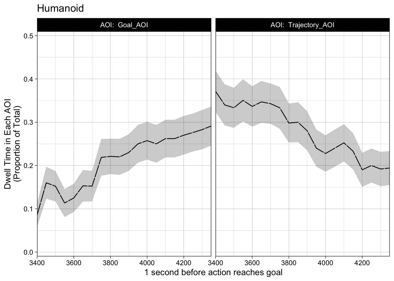
Humanoid visual time sequence

Code

#Humanoid Arm Time Sequence 
time_sequence_data |> group_by(participant) |> filter(motion_type == "Biological") |> filter(agent == "Humanoid") |> 
plot() + theme_linedraw() + coord_cartesian(ylim = c(0,0.5)) + 
  scale_x_continuous(name = "1 second before action reaches goal", expand = c(0,0)) +
  scale_y_continuous(name = "Dwell Time in Each AOI\n(Proportion of Total)", expand = c(-.02,0.02)) + ggtitle("Humanoid")

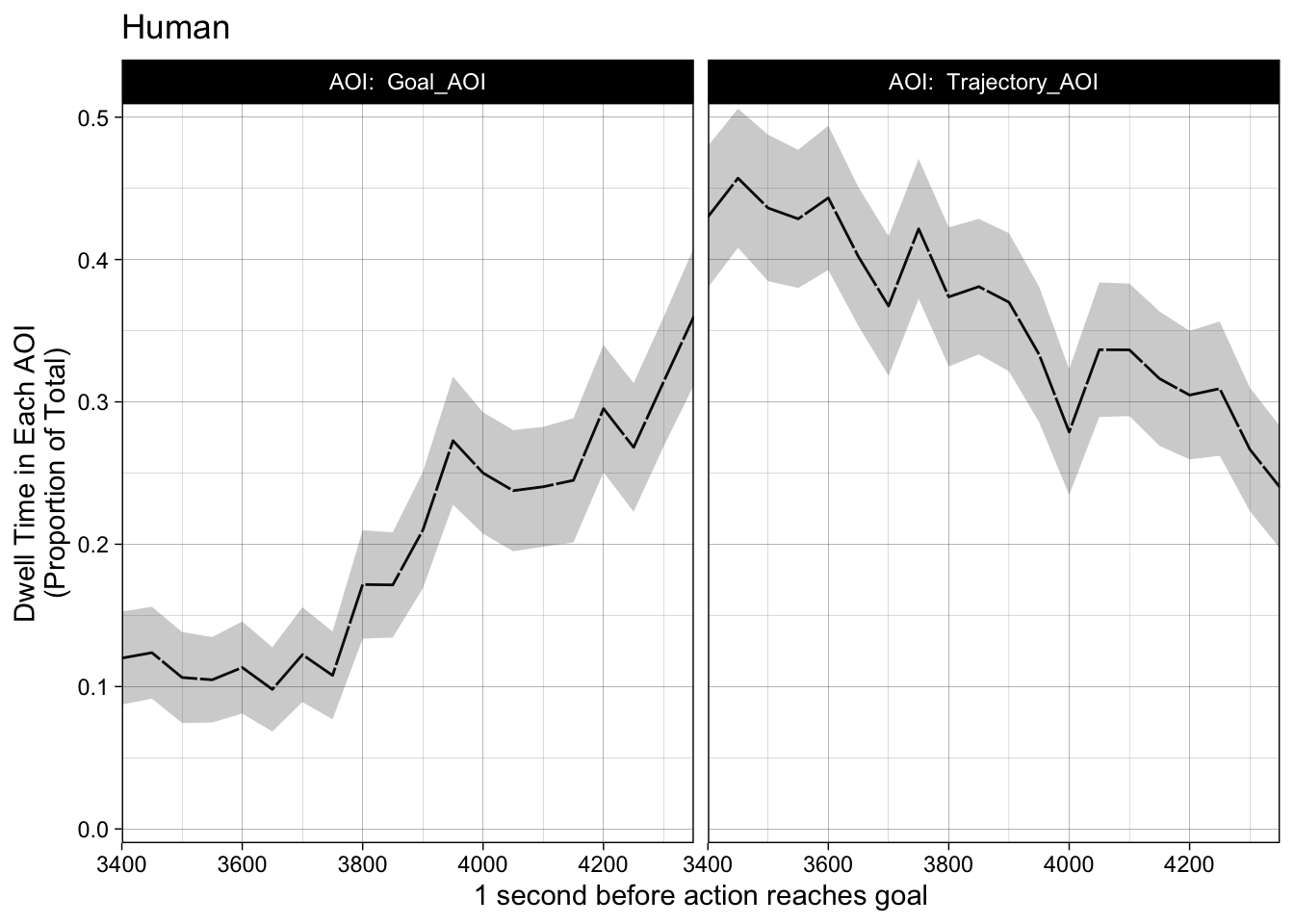
Human Visual Time Sequence

Code

#Human Time Sequence 
time_sequence_data |> group_by(participant) |> filter(motion_type == "Biological") |> filter(agent == "Human") |> 
plot() + theme_linedraw() + coord_cartesian(ylim = c(0,0.5)) + 
  scale_x_continuous(name = "1 second before action reaches goal", expand = c(0,0)) +
  scale_y_continuous(name = "Dwell Time in Each AOI\n(Proportion of Total)", expand = c(-.02,0.02)) + ggtitle("Human")

Aggregate: Calculate predictive gaze

Code

time_window_aggregate <- time_window_data |> 
  select(c(participant, agent, motion_type, trial_index, SamplesInAOI, AOI)) |> 
  group_by(participant, agent, motion_type, trial_index, AOI, SamplesInAOI) |> 
  summarise() |> 
  pivot_wider(names_from = "AOI", values_from = "SamplesInAOI") |> 
  mutate(predictive = Goal_AOI / (Goal_AOI + Trajectory_AOI) ) |> 
  # in the data, NaN denotes that both AOIs had 0 gaze, we convert to NA
  mutate(predictive = ifelse(is.nan(predictive), NA, predictive)) |> 
  # replace all infinity to 5
  # when infinity, gaze was recorded only on Goal AOI, but none on Trajecotry AOI
  # this means the participant was fixated on the Goal and not looking at the movement
  # too many decimal points can't see anything
  mutate(across(where(is.numeric), round, 3))

# exclude due to not looking: V015, V032, V041
# exclude due to fixating only on Goal: V050
time_window_aggregate <- time_window_aggregate |> filter(!participant %in% c("V015", "V029", "V032", "V041", "V050"))

analyse <- time_window_aggregate

# check how many participants had too many NAs (over 6 videos in which they did not look at either of our AOIs)
# count_participants_not_looking <- time_window_aggregate |> group_by(participant, trial_index) |>
#   filter(is.na(predictive)) |> group_by(participant) |> count() |> 
#   filter(n > 7)

# exclude participants
# analyse <- time_window_aggregate |> filter(!participant %in% c(count_participants_not_looking$participant))

# knitr::kable(count_participants_not_looking, align = "c", 
#              caption = "Participants excluded for not looking at any of our AOIs")

Check participants who failed to look at both AOIs

Code

check_not_looking <- count_participants_not_looking$participant

Check participants who fixated only on the Goal AOI

Code

explore_infinity <- analyse |> filter(predictive == 1) |> group_by(participant) |> count()

check_infinity <- explore_infinity$participant

# exploring - how many infinity
# explore_infinite <- analyse |> filter(is.infinite(predictive)) |>
#   group_by(participant) |> count()
# explore_infinite |> filter(n > 6)

# Infinity processed into NA
# 2 more people are excluded because for over 9 of 12 trials, they fixated only on the goal, and not on the trajectory
# analyse <- analyse |> mutate_if(is.numeric, ~replace(., is.infinite(.), NA))

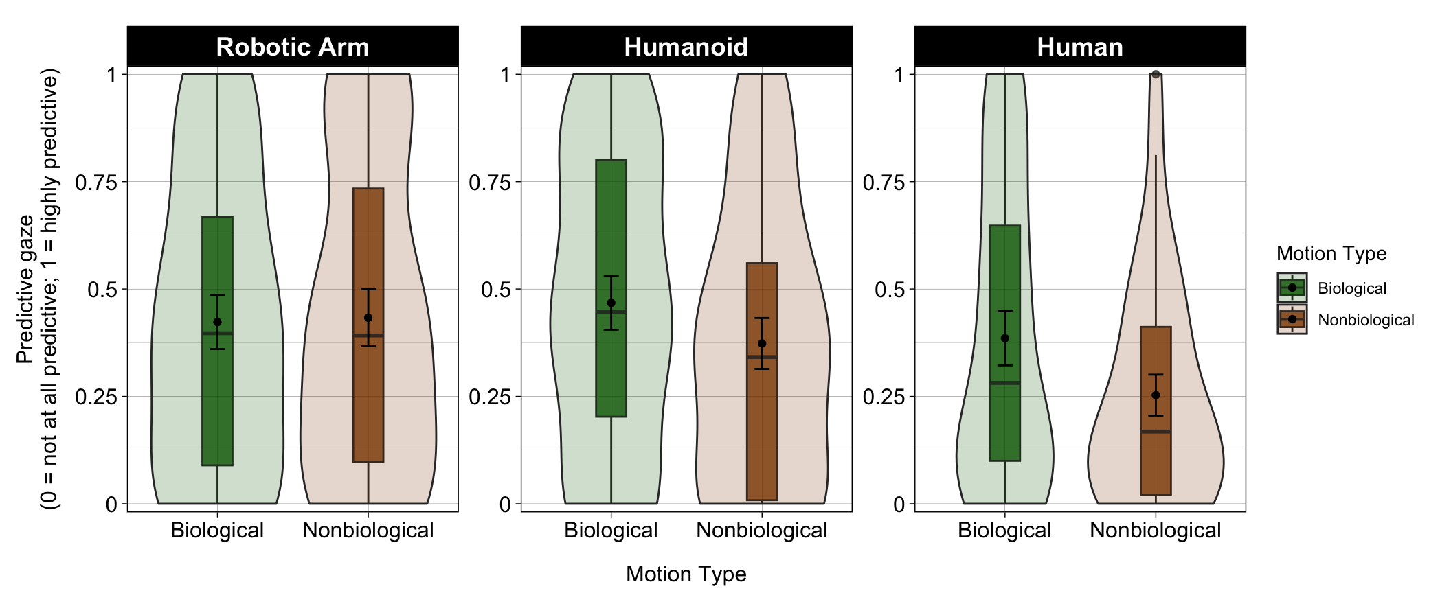
Mean Predictive Gaze calculated here

(Looks to Goal) / (Looks to Goal) + (Looks to Trajectory) if people are only fixated on the trajectory, we expect this to be close to 0 if people are fixated on the goal, it will be close to 1.

Code

analyse_mean <- analyse |> group_by(participant, agent, motion_type) |> 
  mutate(mean_pred = mean(predictive, na.rm = TRUE)) |> 
  select(participant, agent, motion_type, mean_pred) |> distinct() |>
  mutate(across(mean_pred, ~replace_na(., mean(., na.rm=TRUE)))) |>
  mutate(condition = paste(agent, motion_type, sep = ' '))

Visualise

Code

# Function to create the half violin (ref: https://psyteachr.github.io/quant-fun-v2/visualisation.html, section 13.10.2)

"%||%" <- function(a, b) {
  if (!is.null(a)) a else b
}

geom_flat_violin <- function(mapping = NULL, data = NULL, stat = "ydensity",
                             position = "dodge", trim = TRUE, scale = "area",
                             show.legend = NA, inherit.aes = TRUE, ...) {
  layer(
    data = data,
    mapping = mapping,
    stat = stat,
    geom = GeomFlatViolin,
    position = position,
    show.legend = show.legend,
    inherit.aes = inherit.aes,
    params = list(
      trim = trim,
      scale = scale,
      ...
    )
  )
}

GeomFlatViolin <-
  ggproto("Violinist", Geom,
          setup_data = function(data, params) {
            data$width <- data$width %||%
              params$width %||% (resolution(data$x, FALSE) * 0.9)
            
            # ymin, ymax, xmin, and xmax define the bounding rectangle for each group
            data %>%
              group_by(group) %>%
              mutate(ymin = min(y),
                     ymax = max(y),
                     xmin = x,
                     xmax = x + width / 2)
            
          },
          
          draw_group = function(data, panel_scales, coord) {
            # Find the points for the line to go all the way around
            data <- transform(data, xminv = x,
                              xmaxv = x + violinwidth * (xmax - x))
            
            # Make sure it's sorted properly to draw the outline
            newdata <- rbind(plyr::arrange(transform(data, x = xminv), y),
                             plyr::arrange(transform(data, x = xmaxv), -y))
            
            # Close the polygon: set first and last point the same
            # Needed for coord_polar and such
            newdata <- rbind(newdata, newdata[1,])
            
            ggplot2:::ggname("geom_flat_violin", GeomPolygon$draw_panel(newdata, panel_scales, coord))
          },
          
          draw_key = draw_key_polygon,
          
          default_aes = aes(weight = 1, colour = "grey20", fill = "white", size = 0.5,
                            alpha = NA, linetype = "solid"),
          
          required_aes = c("x", "y")
  )

Code

# impute grand mean to those outliers at 1.5 

median(analyse_mean$mean_pred, na.rm = TRUE) #0.3456667

[1] 0.3456667

Code

mean(analyse_mean$mean_pred, na.rm = TRUE) #0.3892676

[1] 0.3892676

Code

analyse_mean |> 
  #  mutate(condition = factor(condition, 
  #                           levels=c("Robotic Arm Biological", 
  # "Robotic Arm Nonbiological", "Humanoid Biological", 
  # "Humanoid Nonbiological", "Human Biological", 
  # "Human Nonbiological"))) |>
  mutate(agent = factor(agent, levels = c("Robotic Arm", "Humanoid", "Human"))) |> 
  ggplot(aes(x = condition, y = mean_pred, fill = motion_type)) +
#  geom_jitter(width = .2, size = 1, alpha = .9, show.legend = FALSE) +
  geom_boxplot(width = .2, alpha = 0.8) +
  geom_violin(alpha = .2, trim = TRUE) +
  stat_summary(fun = "mean", geom = "point") +
  stat_summary(fun.data = "mean_se", geom = "errorbar", width = .1) +
  scale_x_discrete(name = "Motion Type", labels = c("Biological", "Nonbiological")) +
  scale_y_continuous(name = "Predictive gaze\n(0 = not at all predictive; 1 = highly predictive)", limits = c(0, 1),
                      expand = c(0.02, 0, .02, 0), 
                     labels = c("0", "0.25", "0.5", "0.75", "1")
                     ) +
    theme_linedraw() + 
    theme(plot.margin = margin(.5,.5,.5,.5, "cm"), 
        axis.title.x = element_text(size = 12, vjust = -3), 
        axis.title.y = element_text(size = 12, vjust = +3),
        axis.text=element_text(size=12), 
        strip.text = element_text(size = 14, face = "bold")
    ) + facet_wrap(~agent, scales = "free") +
  scale_fill_manual(values = c("darkgreen",  "darkorange4"), 
                    name = "Motion Type")

Code

#write_csv(analyse_mean, "predictiveGaze_aggregate.csv")

Code

analyse_mean |> 
   mutate(condition = factor(condition,
                            levels=c("Robotic Arm Biological",
  "Robotic Arm Nonbiological", "Humanoid Biological",
  "Humanoid Nonbiological", "Human Biological",
  "Human Nonbiological"))) |>
  mutate(agent = factor(agent, levels = c("Robotic Arm", "Humanoid", "Human"))) |> 
  ggplot(aes(x = condition, y = mean_pred, fill = agent)) +
#  geom_jitter(width = .2, size = 1, alpha = .9, show.legend = FALSE) +
  geom_boxplot(width = .2, alpha = 0.8) +
  geom_violin(alpha = .2, trim = TRUE) +
  stat_summary(fun = "mean", geom = "point") +
  stat_summary(fun.data = "mean_se", geom = "errorbar", width = .1) +
  scale_x_discrete(name = "Agent", labels = c("Robotic Arm", "Humanoid", "Human")) +
  scale_y_continuous(name = "Predictive gaze\n(0 = not at all predictive; 1 = highly predictive)", limits = c(0, 1),
                      expand = c(0.02, 0, .02, 0), 
                     labels = c("0", "0.25", "0.5", "0.75", "1")
                     ) +
    theme_linedraw() + 
    theme(plot.margin = margin(.5,.5,.5,.5, "cm"), 
        axis.title.x = element_text(size = 12, vjust = -3), 
        axis.title.y = element_text(size = 12, vjust = +3),
        axis.text=element_text(size=12), 
        strip.text = element_text(size = 14, face = "bold")
    ) + facet_wrap(~motion_type, scales = "free", nrow = 2) +
  scale_fill_manual(values = wes_palette("Cavalcanti1", n = 3), name = "Agent")

Violin

Code

analyse_mean |> 
  mutate(agent = factor(agent, levels = c("Robotic Arm", "Humanoid", "Human"))) |> 
  ggplot(aes(x = condition, y = mean_pred, fill = motion_type)) +
#  geom_jitter(width = .2, size = 1, alpha = .9, show.legend = FALSE) +
  geom_boxplot(width = .3, alpha = 0.5) +
  stat_summary(fun = "mean", geom = "point") +
  stat_summary(fun.data = "mean_se", geom = "errorbar", width = .1) +
  scale_x_discrete(name = "Motion Type", labels = c("Biological", "Nonbiological")) +
  scale_y_continuous(name = "Predictive gaze\n(0 = not at all predictive; 1 = highly predictive)", limits = c(0, 1),
                      expand = c(0.02, 0, .02, 0), 
                     labels = c("0", "0.25", "0.5", "0.75", "1")
                     ) +
    theme_linedraw() + 
    theme(plot.margin = margin(1,1,1,1, "cm"), 
        axis.title = element_text(size = 12),
        axis.text=element_text(size=12), 
        legend.position="none", 
        strip.text = element_text(size = 14, face = "bold")
    ) + facet_wrap(~agent, scales = "free") +
  scale_fill_manual(values = c("darkgreen",  "darkorange4"))

Check Not Looking and Infinity

Code

ALL_time_aggregate <- ALL_time_data |> 
  select(c(participant, agent, motion_type, trial_index, SamplesInAOI, AOI)) |> 
  group_by(participant, agent, motion_type, trial_index, AOI, SamplesInAOI) |> 
  summarise() |> 
  pivot_wider(names_from = "AOI", values_from = "SamplesInAOI") |> 
  mutate(predictive = Goal_AOI / (Goal_AOI + Trajectory_AOI) )

CHECK_infinity <- ALL_time_aggregate |> filter(participant %in% check_infinity)
# exclude 1 person V050 for fixating in the Goal AOI and not looking at the Trajectory AOI at all during 10 of 18 trials

CHECK_not_looking <- ALL_time_aggregate |> filter(participant %in% check_not_looking)
#biggest offenders are: 
# V006 - 7 trials
# V015 - 8 trials
# V032 - 12 trials
# V041 - 11 trials
# exclude the latter 3 participants: V015, V032, V041

Across 6 stimuli, everyone’s gaze between 1500ms before pouring and 500ms after pouring

Colours represent 3 different blocks.

Code

labels_correct<- c("TheoBioCorrect" = "Robotic Arm\nBiological\nCorrect", 
                   "TheoNonbioCorrect" = "Robotic Arm\nNonbiological\nCorrect", 
                   "MiloBioCorrect" = "Humanoid\nBiological\nCorrect", 
                   "MiloNonbioCorrect" ="Humanoid\nNonbiological\nCorrect", 
                   "HumanBioCorrect" = "Human\nBiological\nCorrect",
                   "HumanNonbioCorrect" = "Human\nNonbiological\nCorrect"
)

a <- equal_bins |> 
  group_by(participant, stimulus, interval) |> 
 filter(time > (pour_bin - 1500) & time <= (pour_bin + 500)) |>  
 mutate(stimulus = factor(stimulus, levels= c("TheoBioCorrect","TheoNonbioCorrect", "MiloBioCorrect", "MiloNonbioCorrect", "HumanBioCorrect", "HumanNonbioCorrect")
                             )) |> 
  ggplot() +
  geom_rect(aes(xmin = 605, xmax = 851, ymin = 279, ymax = 567.5), color = "#5E82C9", fill = NA) +
  geom_point(aes(x = x.binned, y = y.binned, color = block), size=0.4) +
  coord_fixed() +
  theme_bw() +
  theme(
    plot.title = element_text(size = 14, face = "bold")
  ) +
  scale_x_continuous(limits = c(1, 1080)) + 
  scale_y_reverse(limits = c(607.5, 1)) +
  scale_colour_manual(values = c("1" = "gray", "2" = "purple", "3" = "orange")) + 
  facet_wrap(~stimulus, labeller = as_labeller(labels_correct), ncol = 2) +
  transition_time(time) + labs(title = "{plyr::round_any(frame_time,50,floor)} ms")

# animate(a, fps = 2, end_pause = 10)

Equal Time Bins of 20ms

Code

# create vector where the bins of 50ms each 
# total length of videos were 7999ms
# v20 <- seq(1, 8000, by = 20)
# v20_intervals <- as_tibble(cbind(v20, findInterval(v20, v20)))

# using findInterval in baseR to match the timestamp from the raw data to the interval in v
# timestamps between 1 and 50 will become 1 in `interval`, etc.
# equal_bins_20 <- eyetrack_data |> 
#   mutate(interval = findInterval(t, v20), .after = t) |>
#   group_by(participant, stimulus, trial_index, interval) |>
#   # mean of x, y coordinates within same tin bin
#   mutate(x.binned = mean(x.adjusted, na.rm = TRUE), .before = t) |> 
#   mutate(y.binned = mean(y.adjusted, na.rm = TRUE), .before = t) |> 
#   # remove the raw data columns
#   select(-c(x.adjusted, y.adjusted, t))|> 
#   # get unique row
#   distinct() |> 
#   # map the interval 1, 2, 3... back into milliseconds 1, 51, 101... 
#   left_join(v_intervals, join_by("interval" == "V2")) |>
#   rename(time = v) |> 
#   left_join(frame_before_outcome, by = "stimulus") |> 
#   # round the pouring moment down to the nearest bin of 50
#   mutate(pour_bin = plyr::round_any(pour_moment,50,floor) + 1) |> 
#   #convert trial_index into block 1, block 2, block 3
#   mutate(block = case_when(trial_index < 7 ~ "1", 
#                                               trial_index > 12 ~ "3", 
#                                               TRUE ~ "2"), .before = stimulus)

Exploring how to filter the noisy data

For Mould’s methods, see ([Mould et al., 2012](https://doi.org/10.1016/j.visres.2011.12.006)). Underlying Mould are Loess smoothers, and my data is too sparse for that.

For dispersion algorithms (see [Blignaut (2009)](https://link.springer.com/content/pdf/10.3758/APP.71.4.881.pdf). Making assumption that everyone was 60cm away from screen. Visual angle for fixations set at .9 degrees (default value set in function).

Code

play <- equal_bins |> mutate(distance = 600) |> select(-c(block, interval, Goal_AOI, Trajectory_AOI, pour_moment, pour_bin))

q <- as.data.frame(play) |> gazepath(x1 = "x.binned", y1 = "y.binned", d1 = "distance", trial = "trial_index", height_px = 607.5, width_px = 1080, height_mm = 160.7, width_mm = 285.75, extra_var = c("participant"),
res_x = 1080, res_y = 607.5, samplerate = 20, method = "MouldDur", posthoc = TRUE, thres_dur = 100, in_thres = 150
)

plot(q, trial_index = 10, fixations_only = TRUE)